Frankenstein (Part 2): Exploring Percy's contribution
Introduction
In my previous post, I described how I created hand annotation files from an existing, manually digitized, richly annotated, draft version of Frankenstein. As I explained in that post, I needed those annotations as a baseline for an authorship attribution analysis of Frankenstein; Would such a machine learning approach come to similar conclusions in terms of Percy Shelley’s contribution to his wife’s famous novel? This article will make a first attempt at answering that question. But first let’s take a closer look at our hand annotation files and see how much and what Percy actually contributed.
Descriptive statistics of Percy’s contribution
First of all we’ll need to import both the tokenized text of Frankenstein and the corresponding hand annotations in a statistics program. I’m using R because it’s free and programmable. We can use it to see how many words were edited or added by Percy.
library(rjson)

text_tokens = fromJSON(file = "./text_list_processed.json")
hand_tokens = fromJSON(file = "./hand_list_processed.json")

hand_df = data.frame(text_tokens, hand_tokens)
num_pbs_words = NROW(hand_df[hand_df$hand_tokens == "pbs",])
prop_pbs_words = num_pbs_words / NROW(hand_df)
The code above stores the amount of words that were authored by Percy in num_pbs_words and the proportion of words in Percy’s hand in prop_pbs_words.
> num_pbs_words
[1] 7173
> prop_pbs_words
[1] 0.1149133
This shows that more than 11% of the 62421 words in the Frankenstein draft were penned by Percy. Surprisingly, this is a bit more than the 4000-5000 words estimated by Charles E. Robinson (2008, p. 25), who created the annotated edition on which our own annotations are based. Our estimate might have been more in line with Robinson’s if we had taken into account that although the final pages of Chapter 18 were (re)written in Percy’s hand, much of the text could have been based on an earlier draft by Mary.
As a next step we could take a look at how Percy’s contributions are distributed throughout the draft. In order to do this, we’ll divide the novel into a large number of equally sized stretches of text (so-called samples).
library(zoo)

sample_size = 100
num_samples = length(hand_tokens) %/% sample_size
num_tokens = num_samples * sample_size
culled_hand_tokens = hand_tokens[1:num_tokens]
hand_matrix = rollapply(culled_hand_tokens, sample_size, by = sample_size, c)
hand_groups = split(hand_matrix, row(hand_matrix))
Now we’ll count for each sample how many words were written by Percy and plot the results.
pbs_proportions = sapply(hand_groups, function(x) sum(x == "pbs"))
plot(pbs_proportions, ylim = c(0,100), type = 'l',
     main = "Percy's contribution throughout Frankenstein",
     xlab = "Sample index (Sample size = 100 words)",
     ylab = "% of words in Percy's hand")
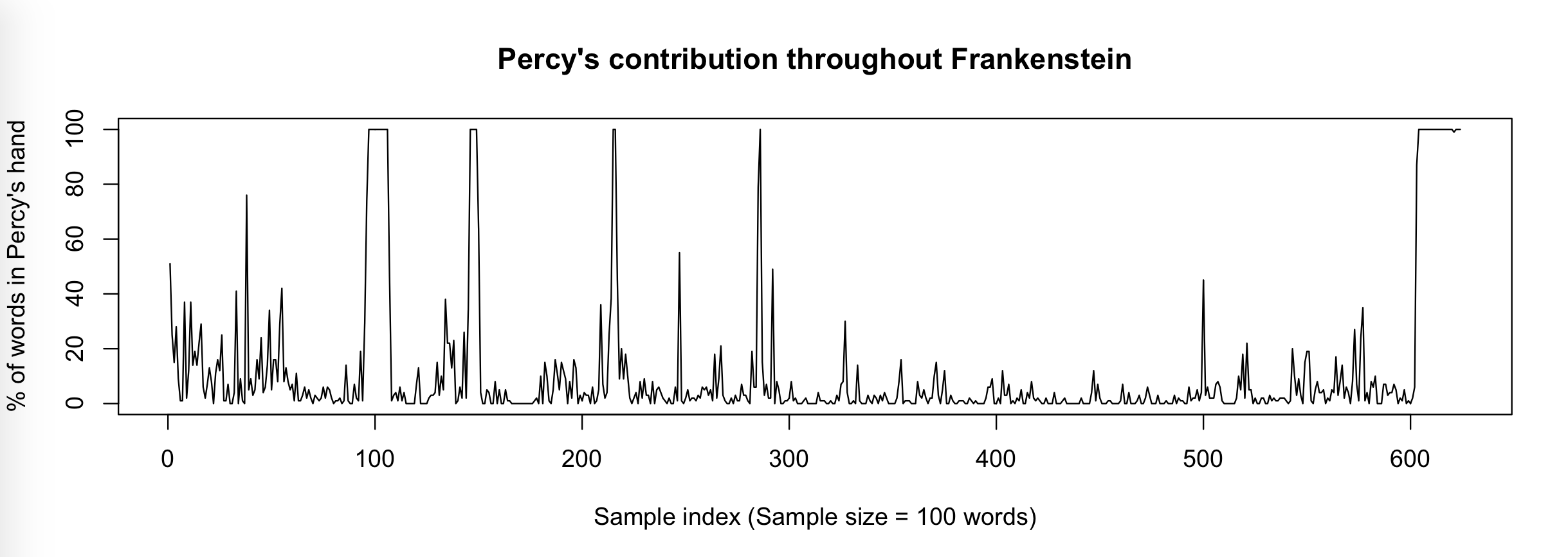 Figure 1
This plot shows that Percy contributed both shorter additions (represented by the smaller spikes) and longer (> 100 words) stretches of text (around index 100, 150 and 600 for example).
We can use our non-tokenized hand annotation files to further investigate the distribution of shorter and longer stretches of consecutive text in Percy’s hand.
text_stretches = fromJSON(file = "./text_list.json")
hand_stretches = fromJSON(file = "./hand_list.json")
stretches_df = data.frame(text_stretches, hand_stretches)
stretches_df$tokens = regmatches(stretches_df$text_stretches,
                                 gregexpr("[a-zA-Z0-9&]+",
                                          stretches_df$text_stretches, perl = TRUE))
stretches_df$num_words = sapply(stretches_df$tokens, function(x) length(x))
Before we can plot the histogram, we’ll need to take the logarithm of word length because Percy contributions could be both very short and very long. We’ll also adjust the x-axis labels accordingly.
stretches_df$num_words_log = log10(stretches_df$num_words)
hist(stretches_df[stretches_df$hand_stretches == "pbs",]$num_words_log,
     xlab = "Contribution length (words)",
     main = "Histogram of PBS contribution lengths", axes = FALSE)
axis(1, labels = seq(0, 3.5, 0.5), at = seq(0, 3.5, 0.5), cex.axis = 0.8, padj = -0.8)
axis(1, labels = rep(10, 8), at = seq(0, 3.5, 0.5), hadj = 1.25, padj = 0.5)
axis(2, labels = seq(0, 600, 100), at = seq(0, 600, 100))
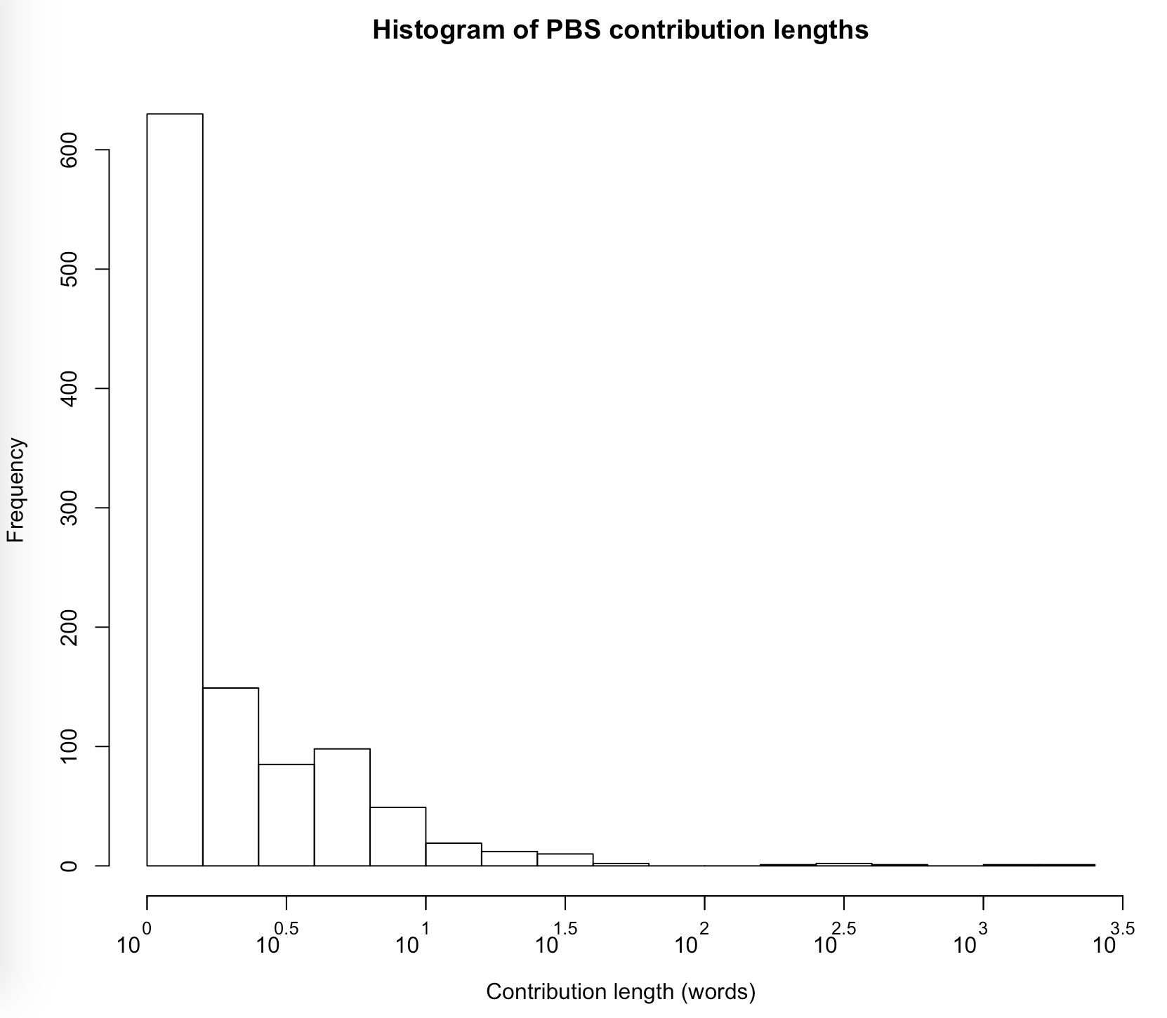 Figure 2
As the histogram shows the overwhelming majority of Percy’s additions consisted of a single word or a few words. However, there were also a few additions of more than a 1000 words. If we make a somewhat arbitrary distinction between short (< 100 words) and long (>= 100 words) contributions, we can calculate the percentage of words in Percy’s hand that were part of a shorter contribution:
short_stretches = sum(stretches_df[stretches_df$hand_stretches == "pbs" & stretches_df$num_words < 100,]$num_words)
long_stretches = sum(stretches_df[stretches_df$hand_stretches == "pbs" & stretches_df$num_words >= 100,]$num_words)
> short_stretches / (short_stretches + long_stretches)
[1] 0.4113602
This shows that even though most of Percy’s contributions were shorter, they only made up about 41% of all text in Percy’s hand.
Now let’s take a look at what Percy’s contributions mostly consist of. For a start, we could look for the words that are used much more frequently by one author compared to the other. We shouldn’t just look at the raw numbers, though. After all, Percy only contributed about 11% of all words. We can take this into account by dividing the raw word counts for each author by their respective total number of words contributed.
mws_freqs = as.data.frame(table(hand_df[hand_df$hand_tokens == "mws",]$text_tokens))
mws_freqs = mws_freqs[order(-mws_freqs$Freq),]
mws_freqs$relFreq = mws_freqs$Freq / table(hand_tokens)["mws"]
names(mws_freqs) = c("word", "MWSFreq", "MWSrelFreq")
pbs_freqs = as.data.frame(table(hand_df[hand_df$hand_tokens == "pbs",]$text_tokens))
pbs_freqs = pbs_freqs[order(-pbs_freqs$Freq),]
pbs_freqs$relFreq = pbs_freqs$Freq / table(hand_tokens)["pbs"]
names(pbs_freqs) = c("word", "PBSFreq", "PBSrelFreq")
all_freqs = merge(mws_freqs, pbs_freqs, by.x = "word", by.y = "word")
all_freqs$freqdif = all_freqs$PBSrelFreq - all_freqs$MWSrelFreq
all_freqs$absfreqdif = abs(all_freqs$freqdif)
all_freqs = all_freqs[order(-all_freqs$absfreqdif),]
After sorting by absolute frequency differential, we can look at the first five rows of all_freqs to see which words can clearly be associated with one author over the other.
> head(all_freqs[, c(1, 3, 5, 6)], 5)
      word  MWSrelFreq PBSrelFreq      freqdif
6336 which 0.005810165 0.01645058  0.010640413
261    and 0.041377063 0.03136763 -0.010009435
5758   the 0.056128729 0.04698174 -0.009146992
2894     i 0.041033160 0.03373763 -0.007295532
3960    of 0.033069070 0.03764115  0.004572084
Note that this way of calculating frequency differences favours authorial differences in very frequent words such as and, the, and I, all of which are used less frequently by Percy. This inherent bias of the difference measure makes it even more striking that which, a less frequent word for both authors, shows the largest difference, with Percy using it more often.
We’re starting to get a better picture of Percy’s additions, but if we want to dig deeper, we will need more sophisticated statistical methods.
Principle Component Analysis 1
One aspect of PCA that makes it more sophisticated is that it allows us to look at what separates Percy’s additions from Mary’s writing in granular detail. In other words, it may find distinctive words in those longer stretches of text that were penned by Percy.
We’ll use a slightly larger sample size this time. As we’ll see, PCA works better with larger samples.
sample_size = 400
num_samples = length(text_tokens) %/% sample_size
num_words = num_samples * sample_size
culled_word_tokens = text_tokens[1:num_words]
word_matrix = rollapply(culled_word_tokens, sample_size, by = sample_size, c)
word_groups = split(word_matrix, row(word_matrix))
Now we’ve split up the tokenized text into samples of 400 words, we need to assign the author labels according to the majority hand of each sample.
culled_hand_tokens = hand_tokens[1:num_words]
hand_matrix = rollapply(culled_hand_tokens, sample_size, by = sample_size, c)
hand_groups = split(hand_matrix, row(hand_matrix))
hand_majorities = sapply(hand_groups, function(x) names(which.max(table(x))))
For convenience, we’ll give each sample a name that includes an index number that corresponds to the indices in Figure 1.
sample_labels = paste(hand_majorities, as.character(4*1:num_samples-3), sep = "_")
names(word_groups) = sample_labels
Now we’ve prepared our text it is time to create the feature set that will be used by the PCA. For this analysis, we’ll only use frequent words as our features. However, we shouldn’t just use any frequent words. For example, certain characters’ names will be much more frequent in one part of the book compared to another part. But such a difference would not really indicate any distinction in writing style between Mary and Percy. As such, we’ll only look at the frequency of so-called function words. These words, which include articles (e.g. the, a), pronouns (e.g. which, you), etcetera, usually perform a grammatical function rather than represent a specific meaning. As a result they are not as sensitive to the specific topic at hand.
First, I sorted the words in Frankenstein by frequency, while accounting for the proportion of each author’s contribution.
all_freqs$mfw = (all_freqs$PBSrelFreq + all_freqs$MWSrelFreq) / 2
all_freqs = all_freqs[order(-all_freqs$mfw),]
Subsequently, I went through the sorted words by hand and picked out the function words until I had a list of the 200 most frequent function words. I saved this list in a .json array.
Next, we’ll load this list into R and use it to transform our samples into feature vectors of which the values represent the frequencies of the function words in that sample.
library(stylo)

function_words = fromJSON(file = "./f_words_frankenstein.json")
freqs = make.table.of.frequencies(word_groups, features = function_words)
The make.table.of.frequencies() function from the stylo library takes each sample and counts for each function word in the list how often it occurs in that sample. That number is then turned into a percentage by dividing it by the sample size and multiplying it by 100.
By looking at the first few rows and columns of freqs, we can get a feeling for what the resulting feature vectors are like:
> freqs[1:3, 1:10]
       the    i  and   of   to   my    a that   in  was
mws_1 3.75 1.75 2.75 4.25 3.25 1.75 1.75 1.25 2.25 3.75
mws_5 5.50 2.00 2.50 4.25 3.75 3.75 1.50 2.50 0.75 1.25
mws_9 5.00 3.25 3.50 4.50 3.00 4.75 1.50 0.75 1.50 1.75
The stylo library actually contains functions for PCA and other analyses, but we’ll use R’s built-in PCA function because it is a little more flexible. As such, we need to change the stylo.data object into a standard R dataframe.
samples = as.data.frame(as.matrix.data.frame(freqs))
rownames(samples) = rownames(freqs)
colnames(samples) = colnames(freqs)
Now we are finally ready to do our first PCA. PCA basically looks at each sample as a point in a multidimensional space. In our case, every dimension of that space represents the frequency of one of the 200 function words. The PCA then tries to find new dimensions (based on the existing ones) that best explain the differences between the predetermined classes (samples labelled Mary versus those labelled Percy).
library(ggbiplot)

samples_pca = prcomp(samples, center = TRUE, scale. = TRUE)
ggbiplot(samples_pca, labels = rownames(samples),
         labels = substr(rownames(samples), 5, nchar(rownames(samples))),
         groups = hand_majorities, var.axes = TRUE, var.scale = 0.2,
         varname.adjust = 8, ellipse = TRUE, varname.size = 2)
The resulting figure plots the samples according to the two dimensions (principle components) that best explain the variance. It also shows how the original features (the function words) relate to these two dimensions.
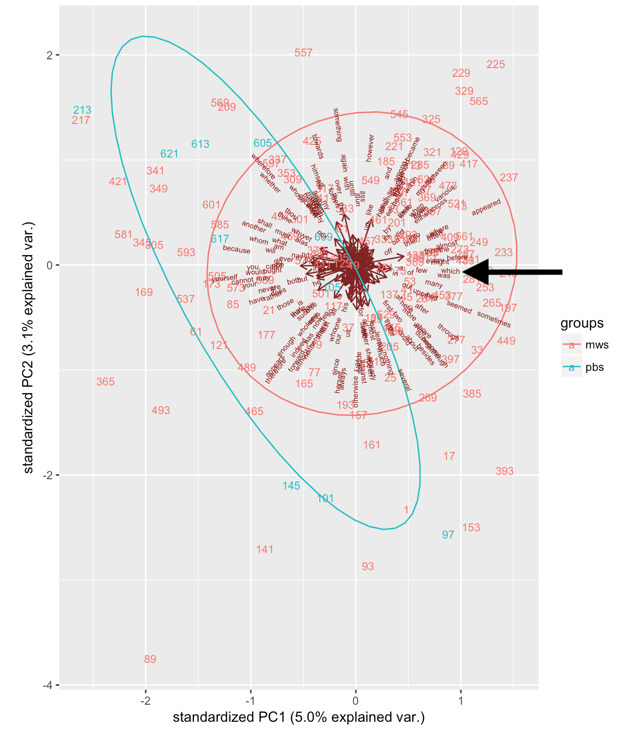 Figure 3
One thing that stands out is how spread out the different samples that were penned by Percy are. In general, Percy’s earlier contributions around index 100 and 150 form a separate cluster from Percy’s later contributions around index 600. This could be explained by the fact that the later samples are from the Fair Copy whereas the earlier samples are from an earlier draft. In other words the earlier samples may represent original contributions by Percy whereas the later sample represent text that was edited by Percy but originally authored by Mary.
Additionally, we can take a look at how our previously established difference between Mary and Percy’s writing, the frequency of the word which, relates to the first two principle components. If we look at the position of which in the plot (see arrow), we can conclude that it is rather strongly related to PC1. Interestingly, however, all of Percy’s samples are located at the opposite end of the plot, which shows that they contain fewer counts of which than most of Mary’s samples. This is the complete opposite of what we would’ve expected from the overall distribution of which. This can only mean that much of Percy’s usage of which consist of additions or changes in stretches of text that were predominantly penned by Mary.
The final thing to note about this plot is that it shows that the PCA wasn’t very successful in separating the samples according to majority hand. This is likely due to the rather small sample size of 400 words.
Principle Component Analysis 2
Unfortunately, we can’t simply increase the sample size to get a more successful separation of Percy’s contributions to Frankenstein. As most of Percy’s longer contributions are only a couple of hundred words long, larger samples would always include a considerable amount of text by Mary.
One way around this problem would be to look at other texts written by Mary and Percy respectively. However, we can’t just use any texts. We need to be sure that the Shelleys did not collaborate on these texts or edited each other’s writing. Percy’s premature death rather simplifies finding material authored solely by Mary. Her first work after the death of husband was the historical novel Valperga, but this work was heavily edited by Mary’s father William Godwin (Rossington, 2000, p. 103). Instead, her next work, the science fiction novel The Last Man, was selected as a suitable text for PCA.
Finding suitable material written by Percy is a bit more difficult. Unfortunately, most of Percy’s later work consists of poetry, which is too different from prose fiction in its structure and diction to be of much use as a training text. However, Percy did publish two novellas, Zastrozzi and St Irvyne, during his time at Eton College and Oxford University in 1810 (O’Neill, 2004). Crucially, he did not start his relationship with William Godwin, which led to his acquaintance with Mary, until January of 1812 (O’Neill, 2004). It can be concluded, then, that Mary had no influence whatsoever on these novellas.
Of course, these texts also have to be prepared for use in a PCA. Fortunately, this process is much easier for these novels than it was for Frankenstein, as we don’t need to keep track of hand changes. I simply downloaded the raw text files from Project Gutenberg and Project Gutenberg of Australia, and turned them into tokenized arrays; the R code below uses the regular expression [a-zA-Z0-9]+ to match all sequences of consecutive lowercase letters, uppercase letters and numbers, that is to say, all words, and put them into an array.
thelastman_text = readChar("./mws_the-last-man.txt", file.info("./mws_the-last-man.txt")$size)
thelastman = tolower(regmatches(thelastman_text, gregexpr("[a-zA-Z0-9]+", thelastman_text, perl = TRUE))[[0]])

stirvyne_text = readChar("./pbs_st-irvyne.txt", file.info("./pbs_st-irvyne.txt")$size)
stirvyne = tolower(regmatches(stirvyne_text, gregexpr("[a-zA-Z0-9]+", stirvyne_text, perl = TRUE))[[0]])

zastrozzi_text = readChar("./pbs_zastrozzi.txt", file.info("./pbs_zastrozzi.txt")$size)
zastrozzi = tolower(regmatches(zastrozzi_text, gregexpr("[a-zA-Z0-9]+", zastrozzi_text, perl = TRUE))[[0]])
After preprocessing the new texts, we can prepare them for PCA in much the same way as we did for Frankenstein. However, this time we’ll use the make.samples() function from the stylo package to sample the texts. We’ll also use a much larger sample size.
training_texts = list(thelastman, stirvyne, zastrozzi)
names(training_texts) = c("mws_the-last-man", "pbs_st-irvyne", "pbs_zastrozzi")

sample_size = 5000
training_samples = make.samples(training_texts, sampling = "normal.sampling", sample.size = sample_size)
Furthermore, we’ll use a different function word list: one that also takes into account the most frequent function words in The Last Man, St. Irvyne and Zastrozzi.
function_words = fromJSON(file = "./f_words_shelleys.json")

training_freqs = make.table.of.frequencies(training_samples, features = function_words)
training_freqs_df = as.data.frame(as.matrix.data.frame(training_freqs))
rownames(training_freqs_df) = rownames(training_freqs)
colnames(training_freqs_df) = colnames(training_freqs)

training_pca = prcomp(training_freqs_df, center = TRUE, scale. = TRUE)
Having done the PCA, we can now plot the results:
author_names = substr(rownames(training_freqs), 1, 3)
num_train_samples = NROW(training_freqs_df)
ggbiplot(training_pca, labels = rep("*", num_train_samples),
         groups = author_names, var.axes = TRUE, var.scale = 0.2,
         varname.adjust = 8, ellipse = TRUE)
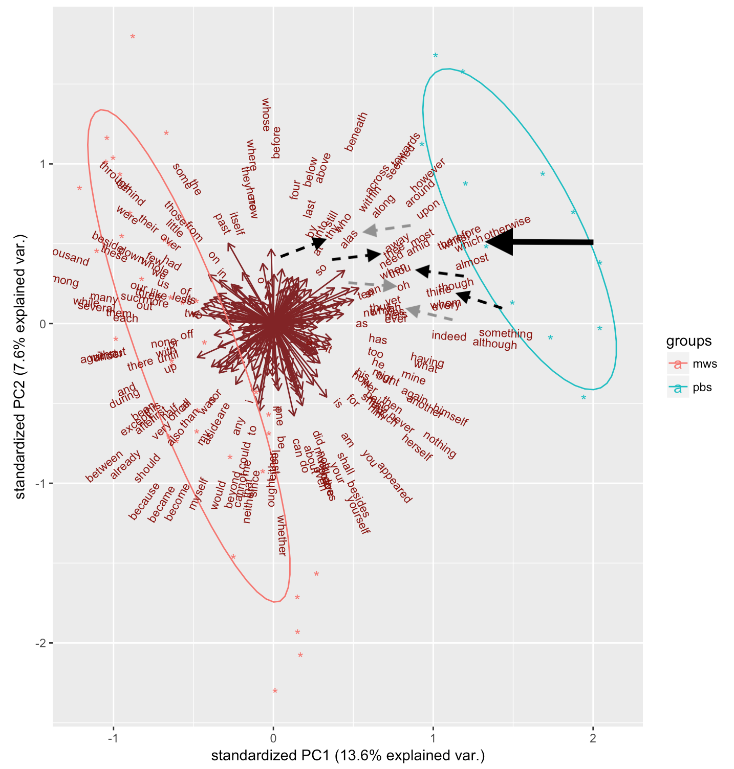 Figure 4
The first thing that stands out is the clear separation between all PBS and MWS samples. This is also reflected in the increased amount of variance explained by the principle components (compared to the first PCA; see Figure 3).
This more successful grouping of the respective authors’ samples also allows us to look for distinctive features of Mary and Percy’s writing styles. First of all, we can confirm our earlier finding that the use of which (see large arrow in Fig. 4) is clearly associated with Percy. Furthermore, the black dashed arrows in Figure 4 indicate a sort of grouping of pronouns that start in th: thy, thee, thou and thine all seem to be more frequent in Percy’s writing compared to Mary’s. Similarly, the grey dashed arrows highlight a number of interjections, ah, oh and alas, that Percy uses more often than Mary
We don’t just have to trust our eyes though. The clear separation on the PC1 axis alone makes it easy to identify influential words by looking at the variable loadings. These can be interpreted as the degree of correlation between the variables (i.e. the function word frequencies) and the principle components. We can take a look at the strongest loadings for PC1 as follows:
rotation_df = as.data.frame(training_pca$rotation)
rotation_df_ordered = rotation_df[order(-abs(rotation_df$PC1)),]
structure(rotation_df_ordered[1:5, "PC1"],
          names=rownames(rotation_df_ordered)[1:5])
     which      while         oh     whilst        and
 0.1621990 -0.1543644  0.1523841  0.1445798 -0.1443804
This confirms much of what we had already identified: which and and are more frequent in Percy and Mary’s writing styles respectively, and Percy tends to use more interjections such as oh.
However, these variable loadings also reveal an alternation that had previously gone unnoticed. Mary seems to have a preference for while, whereas Percy likes to use the more literary whilst. It seems, to me at least, that Percy’s preference for this form goes hand in hand with his use of the more archaic personal pronoun forms. In both cases, the variants preferred by Percy are grammatically more specific. Whilst can only be used as a conjunction or adverb, and thou, thee, and thy/thine still carry nominative, accusative and genitive case respectively.
We need to keep in mind that we have not established yet that the differences in the use of while/whilst, the pronouns and the interjections also play a role in Frankenstein. So let’s take a look at the frequencies in Frankenstein.
First up, the alternation between while and whilst:
hand_df_whil = hand_df[hand_df$text_tokens == "while" | hand_df$text_tokens == "whilst",]
hand_df_whil$text_tokens = factor(hand_df_whil$text_tokens)
hand_df_whil$hand_tokens = factor(hand_df_whil$hand_tokens)
whil_counts = table(hand_df_whil$text_tokens, hand_df_whil$hand_tokens)
whil_counts[, "mws"] = whil_counts[, "mws"] / sum(whil_counts[, "mws"])
whil_counts[, "pbs"] = whil_counts[, "pbs"] / sum(whil_counts[, "pbs"])

barplot(whil_counts, main = "Distribution of 'while' / 'whilst' in Frankenstein",
        ylab = "Hand Annotation", col = c("gray", "white"), xpd = FALSE, xlab = "Proportion of variant",
        legend = rownames(whil_counts), horiz = TRUE, names.arg = colnames(whil_counts),
        args.legend = list(x = "top", horiz = TRUE, inset=c(0, -0.12), xpd = TRUE, bty = "n"))
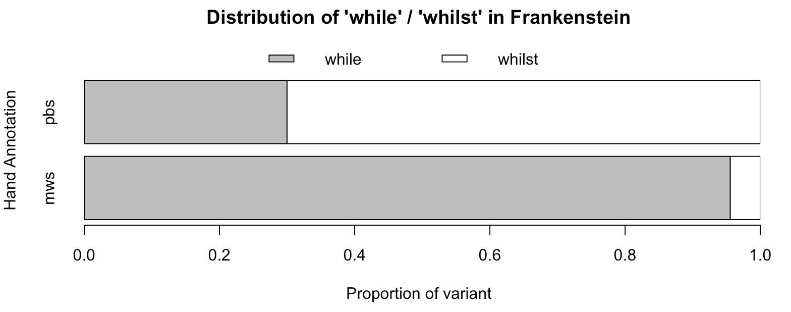 Figure 5
Now let’s take a look at the 2nd person pronouns. I’ll spare you the code this time.
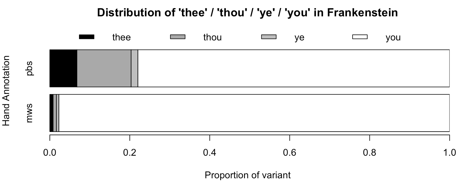 Figure 6a
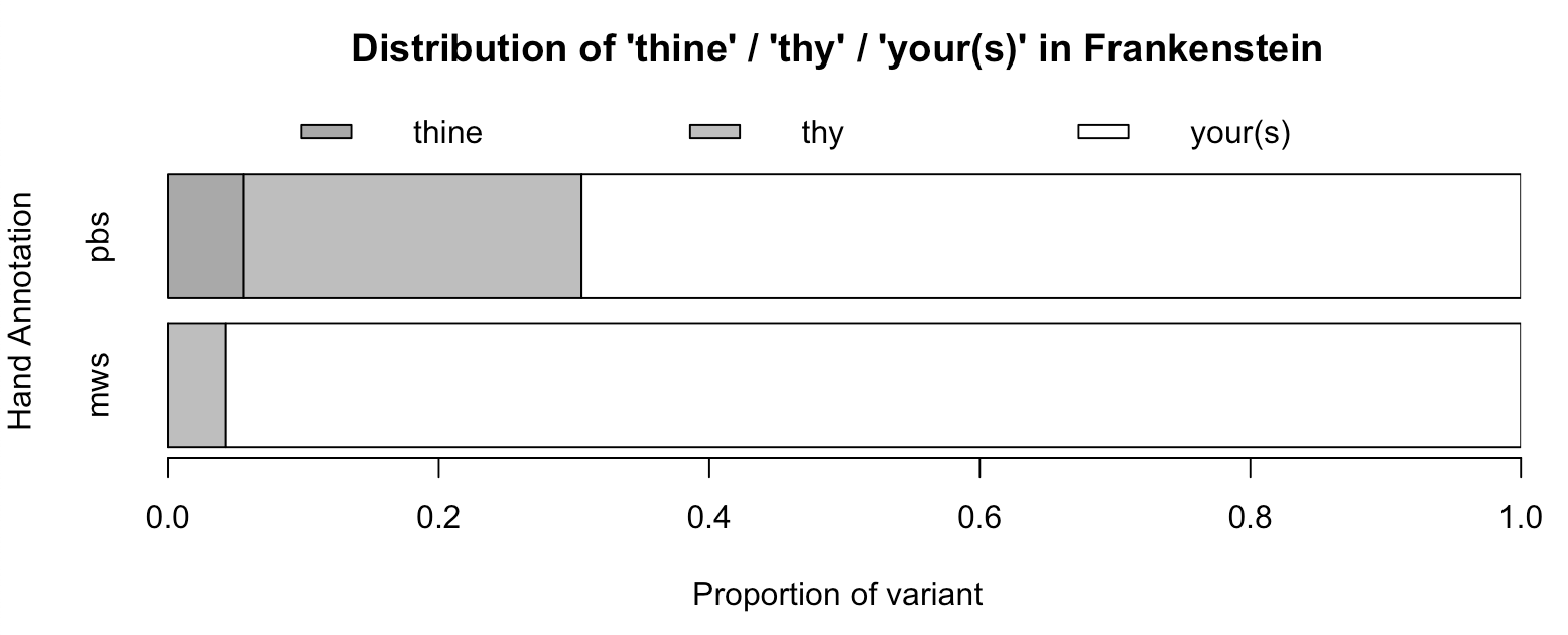 Figure 6b
Finally, we’ll plot the frequencies of the interjections. As these interjections can’t really be contrasted with a standard variant (as was the case in the previous plots), we’ll plot the respective interjection frequencies as percentages of the two authors’ total word counts.
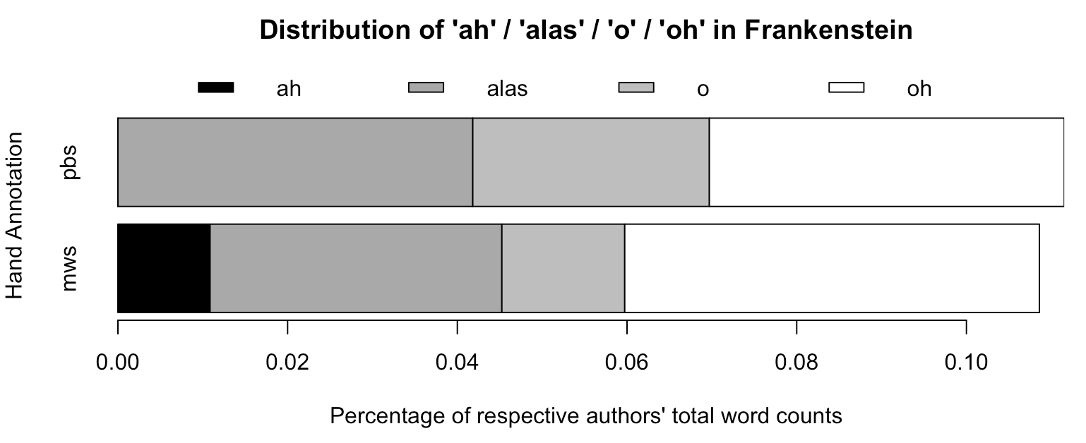 Figure 7
Based on Figures 5 through 7, we can see that apart from the interjections, all of the words that we identified as differentiating Percy and Mary’s other works also play a role in Frankenstein.
However, we still have no clue whether these features can be used to actually differentiate samples of Frankenstein that were mostly penned by Percy. For all we know, these distinctive words were mostly part of smaller additions or corrections in samples that were predominantly written by Mary (as was the case with which).
To find out, we can do something pretty cool; We can project the samples we made for the first PCA, i.e. samples that are 400 words long, on the principle components that were made in our second PCA.
First, we’ll update the feature set to be compatible with the second PCA:
franken_freqs = make.table.of.frequencies(word_groups, features = function_words)
franken_freqs_df = as.data.frame(as.matrix.data.frame(franken_freqs))
rownames(franken_freqs_df) = rownames(franken_freqs)
colnames(franken_freqs_df) = colnames(franken_freqs)
And then we can project these frequencies on the principle components, and plot the projection.
frankenstein_sc = scale(franken_freqs, center = training_pca$center)
frankenstein_pred = frankenstein_sc %*% training_pca$rotation
training_plus_pca = training_pca
training_plus_pca$x = rbind(training_plus_pca$x, frankenstein_pred)
franken_names = paste(substr(rownames(franken_freqs_df), 1, 3),
                      rep("F", num_samples), sep = "-")
franken_nums = substr(rownames(samples), 5, nchar(rownames(franken_freqs_df)))

ggbiplot(training_plus_pca,
         labels = c(rep("*", num_train_samples), franken_nums),
         groups = c(author_names, franken_names), var.axes = TRUE,
         ellipse = TRUE, var.scale = 0.2, varname.adjust = 8, labels.size = 4)
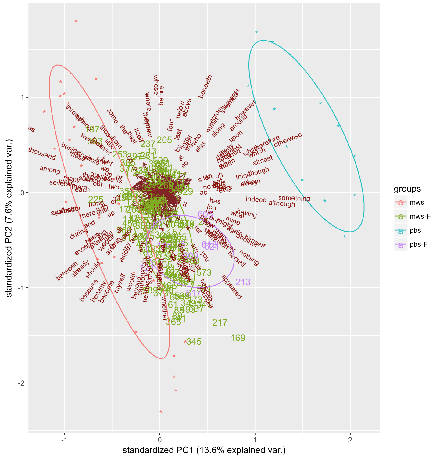 Figure 8
Once again, I’ve given the Frankenstein samples labels that correspond to the indices in Figure 1, so that we have some idea of the location of these samples in the novel.
We can see that, in general, the Frankenstein samples are closer to Mary’s The Last Man samples than Percy’s Zastrozzi and St. Irvyne samples. However, some of the Frankenstein samples that were written in Percy’s hand (see the purple labels in Figure 8) seem to be somewhat separate of the rest, especially along the PC1 axis.
If we take a closer look at one of these samples, we can see that the previously identified distinctive features may play a role in separating it from the bulk of Frankenstein samples. For example, if we take sample 213, and we look at the total amount of archaic pronoun forms, we find the following:
franken_freqs_df$th = franken_freqs_df$thee + franken_freqs_df$thou +
                      franken_freqs_df$thy + franken_freqs_df$thine
> mean(franken_th_df$th) * 4
[1] 0.2564103
> franken_th_df["pbs_213",]$th * 4
[1] 16
In other words, the mean amount of archaic pronouns across all 400-word samples of Frankenstein is much smaller than 1, whereas sample 213 contains 16 archaic pronouns. It seems, then, that in certain cases Percy’s distinctive use of certain words can be used to identify stretches of the Frankenstein draft that were written in his hand.
Conclusion
Using just function word frequencies, it is hard to separate all of Mary and Percy’s contributions to Frankenstein. However, these features can be used to differentiate their styles in general. Percy tends to use more dramatic and literary language. And some longer stretches of Frankenstein that were penned by Percy can definitely be identified as such, using some of the same features.
In a future article, I may look at a more formal way to classify samples of Frankenstein as written by Mary or Percy, based on the training texts we used in the second PCA. Nevertheless, the analysis in this article led to some interesting insights regarding the differences in Mary and Percy’s writing styles.
References
- O’Neill, M. (2004). Shelley, Percy Bysshe (1792–1822). In B. Harrison (Ed.), Oxford Dictionary of National Biography. Retrieved from Oxford University Press. doi:10.1093/ref:odnb/25312.
- Robinson, C.E. (2008). The Original Frankenstein. New York: Vintage Books.
- Rossington, M. (2000). Future uncertain: The republican tradition and its destiny in Valperga. In B.T. Bennett & S. Curran (Eds.), Mary Shelley in Her Times (103-118). Baltimore: Johns Hopkins University Press.